Using Wheatstone Bridges with RTDs

Introduction

Currently, I’m building a circuit to measure temperature using a resistive temperature device (RTD). Like their name implies, RTDs change resistance in response to temperature changes; thus, the accuracy of a RTD setup is dependent on how accurately we can measure resistance. Wheatstone bridges are a low-cost, well-documented pattern for interfacing with resistive sensors like RTDs or strain gauges.

Theory

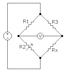
A Wheatstone bridge is best thought of as two voltage dividers wired in parallel, where the voltage between the left and right dividers is zero if the network is balanced. By Ohm’s Law, $V_{L} = Vdd\frac{R_{2}}{R_{1} + R_{2}}$ and $V_{R} = Vdd\frac{R_{x}}{R_{3} + R_{x}}$ . Through basic manipulation, we can write one of the resistor values (such as R2) in terms of $V_{LR}$ and the other resistors. Note that $V_{LR} = V_{L} - V_{R}$ can be positive or negative, depending on the value of R2.

WikiMedia Commons (CC BY-SA 3.0, https://commons.wikimedia.org/w/index.php?curid=80346)

$V_{LR} = Vdd(\frac{R_{2}}{R_{1} + R_{2}} - \frac{R_{x}}{R_{3} + R_{x}})$

$\frac{V_{LR}}{Vdd} + \frac{R_{x}}{R_{3} + R_{x}} = \frac{R_{2}}{R_{1} + R_{2}}$

$(R_{1} + R_{2})(\frac{V_{LR}}{Vdd} + \frac{R_{x}}{R_{3} + R_{x}}) = R_{2}$

$\frac{R_{1}(\frac{V_{LR}}{Vdd} + \frac{R_{x}}{R_{3} + R_{x}})}{1 - (\frac{V_{LR}}{Vdd} + \frac{R_{x}}{R_{3} + R_{x}})} = R_{2}$

$R_{2} = \frac{R_{1}\frac{V_{LR}(R_{3} + R_{x}) + R_{x}Vdd}{Vdd(R_{3} + R_{x})}}{\frac{Vdd(R_{3} + R_{x}) - [V_{LR}(R_{3} + R_{x}) + R_{x}Vdd]}{Vdd(R_{3} + R_{x})}}$

$R_{2} = \frac{R_{1}[V_{LR}(R_{3} + R_{x}) + R_{x}Vdd]}{VddR_{3} - V_{LR}(R_{3} + R_{x})}$

Though simple, this arrangement does not account for lead wire impedance. This is why many RTDs come with a third (or even fourth) wire. It’s possible to use a three-wire RTD with a Wheatstone bridge. In this example, $R_{L}$ indicates the lead impedance, and $R_{g}$ the desired resistance.

Omega Engineering, Inc. (https://br.omega.com/omegaFiles/temperature/z/pdf/z033-035.pdf)

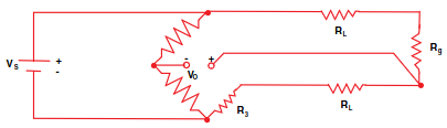
Rather than derive these expressions from scratch (which we could do by repeating the previous process, treating $R_{L}$ and $R_{g}$ and $R_{L}$ and $R_{3}$ as series resistances), we use the published expressions from Omega.

$R_{g} = R_{3}(\frac{V_{s} - 2V_{0}}{V_{s} + 2V_{0}}) - R_{L}(\frac{4V_{0}}{V_{s} + 2V_{0}})$

For our use case, we won’t use the three-wire approach, but it is important to be aware of it.

Callendar–Van Dusen Equation

Now that we have a useful equation to calculate the resistance, we need to convert it to a temperature value. British physicist Hugh Longbourne Callendar proposed a quadratic equation modelling the relationship between temperature and resistance for temperatures above 0 °C.

$R_{t} = R_{0}(1 + At + Bt^{2})$

$R_{0}$ is the resistance at 0 °C, and $A$ and $B$ are constants, typically derived through calibration. For typical industrial RTDs, they are $A = 3.9083 \times 10^{-3} C^{-1}$ and $B = -5.775 \times 10^{-7} C^{-2}$ (EN 60751:1995). See this document from Wika for more information.

For a quick sanity check, let’s see what resistance value this equation generates for a PT100 RTD ( $R_{0} = 100 \Omega$ ) at water boiling temperature (100 °C).

$R_{t} = 100[1 + (3.9083 \times 10^{-3})(100) + (-5.775 \times 10^{-7})(100)^{2}] = 138.5055 \Omega$

Sure enough, published tables put the resistance value at 138.505Ω.

Let’s solve Callendar’s equation to derive the temperature from resistance. Note that this form only works for positive temperatures; Callendar’s equation fails for sub-0 °C temperatures.

$t = \frac{-A + \sqrt{A^{2} - 4B(1 - \frac{R_{t}}{R_{0}})}}{2B}$

American chemist M. S. van Dusen appended a third term to Callendar’s expression to accommodate negative temperatures. Since my application measures room temperature or higher, the quadratic form works sufficiently well, but it is important to be aware of the cubic equation.

$R_{t} = R_{0}(1 + At + Bt^{2} + C(t - 100)t^{3})$

Circuit Construction

Let’s estimate the voltage at the Wheatstone bridge’s terminals at room temperature (~22 °C) when driven with 3.33 V from a lab bench power supply. The PT100 has a resistance of 108.570Ω.

$V_{O} = 3.33(\frac{108.570 \Omega}{108.570 \Omega + 100 \Omega} - \frac{100 \Omega}{100 \Omega + 100 \Omega}) = 68.4 mV$

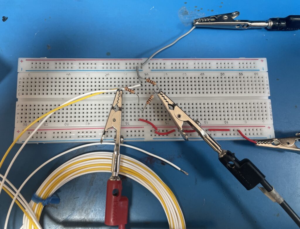
When I built this circuit, I observed 98.8 mV. The temperature of the lab, the use of low-precision resistors (5% tolerance), and the lack of compensation for lead impedance contributed to this sizable discrepancy.

Let’s plug 98.8 mV into our two-lead Wheastone bridge model to calculate resistance.

$R_{2} = \frac{(100 \Omega)[(0.0988 V)(100 \Omega + 100 \Omega) + (100 \Omega)(3.33 V)]}{(3.33 V)(100 \Omega) - (0.0988 V)(100 \Omega + 100 \Omega)} \approx 112 \Omega$

From there, we can generate an approximate temperature using Callendar’s equation.

$t = \frac{-A + \sqrt{A^{2} - 4B(1 - \frac{112.62 \Omega}{100 \Omega})}}{2B} = 32.45 ^{\circ}C = 90.41 ^{\circ}F$

At the very least, it is crucial that we use precision resistors to mitigate errors on the order of $10 ^{\circ}C$ .

Microcontroller Interface

Now that we understand Wheatstone bridges, we would like to use them in our microcontroller projects. One possible barrier is differential signaling: How do we reference the voltage difference between the branches of the Wheatstone bridge relative to the microcontroller’s ground? One approach involves using two analog inputs; implementing this solution will be the subject of our next post.